Quality AnalytiX Quick Start Guide

This topic provides you with the information you need to configure and view an SPC data configuration quickly using Quality AnalytiX. While the steps below cover most of the features available in the product, they do not provide in-depth descriptions. To view more information about a specific aspect in Quality AnalytiX, view the links provided in each of the steps below.

Because it takes several steps to define and view SPC data, this quick start guide contains several sections. Read the sections that are most relevant to you.

To configure and view a basic process quality configuration for Quality AnalytiX:

(Required) Configure your SPC tags in Hyper Historian (Classic).
(Optional) Set up an SPC plot in TrendWorX64 Viewer to show how your configured SPC tags and associated values change over time. You can also view alarm notifications and operator comments associated with your SPC data in this type of plot.
(Optional) Generate reports for viewing sample calculations, group calculations, and alarm calculations associated with your SPC tags.
(Optional) Create a dashboard to display your SPC tags.

Configuring SPC Tags in Hyper Historian (Classic)

Open an active Hyper Historian (Classic) database and expand the folder called SPC Distribution Rules. This folder includes the default set of rule sets in Quality AnalytiX. Each rule set defines the tendencies your SPC tag values should or should not follow. For more information about creating or editing SPC distribution rule sets, see the SPC Distribution Rule Sets topic.
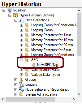
In Hyper Historian, expand the Data Collections folder and create a new folder called SPC. Once you have created this folder, right-click on it and select the + SPC Tag option to create a new SPC tag. The SPC Tag Configuration Dialog appears, and the project explorer contains the SPC folder and your new tag, as shown below:

New SPC Folder and Tag Appearing in Project Explorer

For more information about adding and editing SPC tags in Hyper Historian, follow the steps in the SPC Tags topic.
In the SPC Tag Configuration Dialog, configure the tag using the following options. For more details about the tabs found in this dialog, see the SPC Tag Configuration Dialog topic.
1. Give the tag a Name of Test.
2. In the "Properties" tab of the dialog, assign the following Data Point to this SPC tag: data:LogGrp.OPCUA.Ramp.
3. Select a set of Distribution Rules (such as Basic) for this SPC tag to follow.
4. Select a Collection Type of XBarS to summarize the sample values that this SPC tag measures.
5. In the Chart Properties area of the tab, set the limits of the XBar summary statistic to 110.00 (for a Hi Limit) and -10.00 (for a Lo Limit). Similarly, set the limits of the StdDev summary statistic to 10.00 (for a Hi Limit) and 1.00 (for a Lo Limit).
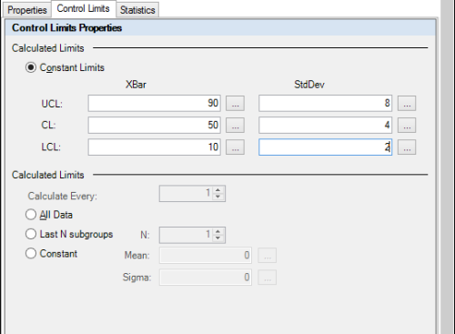
6. Move to the "Control Limits" tab of the dialog. In the Calculated Limits area of the tab, set the XBar values to 90 for UCL, 50 for CL, and 10 for LCL. Set the StdDev values to 8 for UCL, 4 for CL, and 2 for LCL. The following image shows the completed configuration on this tab.
  
  Sample "Control Limits" Configuration
7. Move to the "Statistics" tab of the dialog. In the Process Capability Ratios area of the tab (near the right-hand edge), enable the check boxes next to Cp, Pp, Mean, Sigma, Avg, and StdDev.
8. Click Apply to save the changes you have made to this SPC tag.
Make sure that the Services traffic light that appears in the Home ribbon is green before continuing.

Setting Up an SPC Plot in TrendWorX64 Viewer

Open TrendWorX64 Viewer and create a new trend.
In the TrendWorX64 Viewer Configuration ribbon, select the Configure Viewer button. The TrendWorX Viewer Configurator appears.
In the left navigation tree pane of the TrendWorX64 Viewer Configurator, right-click the Chart element and select Add > Plot.
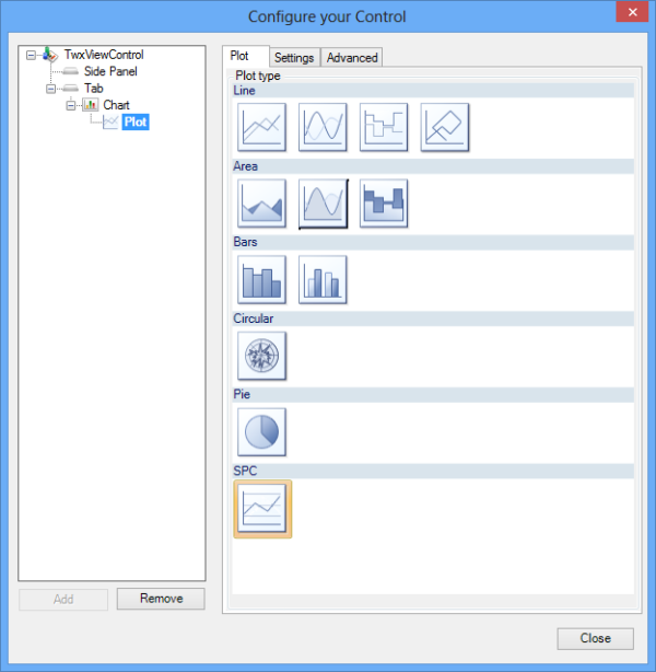
For a plot type, navigate to the SPC plot group and select the plot that appears in this group, as shown in the following image:

Selecting the SPC Plot Type
Open the plot's Settings tab. In the Data area of this tab, enter a Data Source of HyperHistorian\\Configuration/SPC/%Test/Average. You can also browse to this tag using the Data Browser.
In the Appearance area on the Settings tab, enter a descriptive Title for your plot (such as Valve 1 Temperature). For more information about the settings available on this tab, see the Creating an SPC Plot in TrendWorX64 Viewer topic.
Click Close to save your plot settings and return to the main trend display.
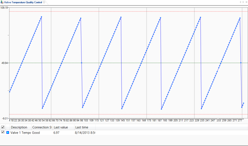
In the top-right corner of the Workbench window, select the Runtime button to begin viewing real-time trending data. An example of the plot as it appears in Runtime mode appears below:

TrendWorX64 Viewer Runtime Mode - SPC Plot Displaying Test Tag Data
You can view operator comments that contain collected or calculated SPC tag values within the main trend display. To learn more about creating and viewing operator comments, see the Runtime Operations in TrendWorX64 Viewer topic.
If your SPC tag values trigger alarms, the plot will contain different point marker colors to represent alarm states. For more information about runtime annotation features, see the SPC Plot Annotation topic.

Generating Reports to Display SPC Tag Calculations

For information about generating reports, see the Quality AnalytiX Reports topic.

Creating a Dashboard of SPC Tag Information

You can create dashboard displays that provide holistic summaries of your SPC information. This visual overview allows you to identify the elements of your process that are affecting its capability and performance. An example appears below:

Sample SPC Dashboard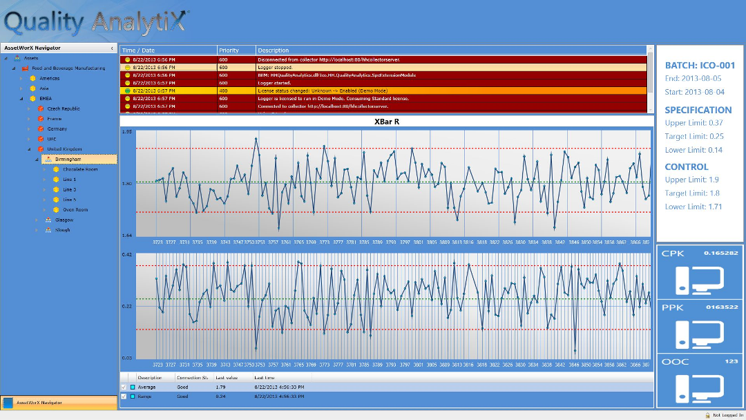

For information about creating dashboards, see the Creating Dashboards for Quality AnalytiX topic.