|
|
The features on this page require a GENESIS64 Advanced license and are not available with GENESIS64 Basic SCADA . |
|
|
The features on this page require a GENESIS64 Advanced license and are not available with GENESIS64 Basic SCADA . |
The AnalytiX-BI Server supports a subset of SQL for running queries against data models. Queries can be provided as part of a point name (see the "Ad Hoc Queries" section of AnalytiX-BI Runtime) or used in a data view.
Below we will detail the different SQL keywords that the AnalytiX-BI Server's query engine supports and how they may differ from standared SQL>
SELECT needs to be followed by a list of attributes, fully qualified as <table name>.<column name>. Table and column names containing reserved symbols (such as spaces, commas, or periods) must be enclosed in square brackets.
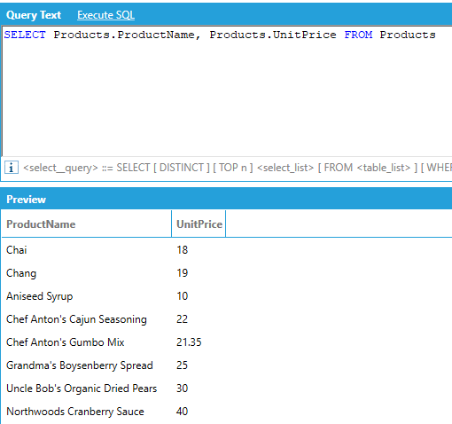
The FROM keyword is optional, as AnalytiX-BI automatically determines the source table(s) from the list of requested attributes. However, the table name must always be included with each column name, even when including the FROM clause.
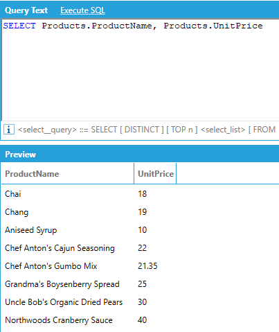
Which is equivalent to:
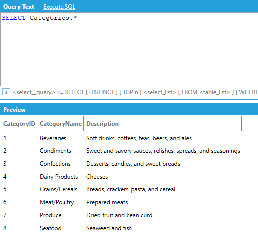
The star or asterisk (*) qualifier can be used to retrieve all the columns of a table. However, when using star, the query is limited to selecting from just one table.
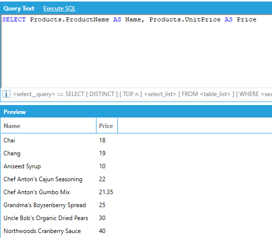
Selected attributes can be aliased in using the AS keyword. The alias is used as the column header in the output. The aliased name can also be used in other clauses, such as WHERE and ORDER BY.
If relationships between tables are established in the data model, the JOIN keyword is optional. AnalytiX-BI can determine the join path among all the tables that are referenced in the list of the SELECT attributes automatically.
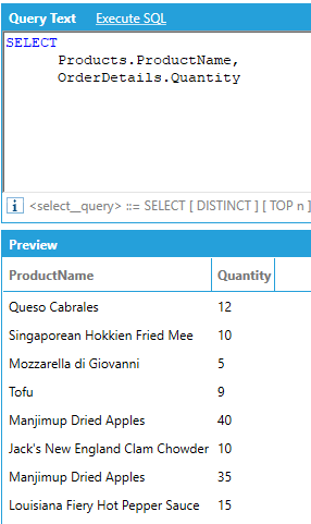
Is equivalent to:
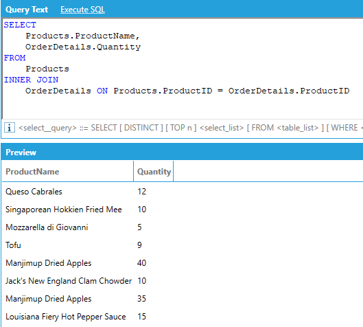
AnalytiX-BI only supports INNER equi-joins (the join condition must be expressed using the equality operator), OUTER joins are not supported.
Note: If relationships in the data model are not established between the requested tables the FROM and JOIN keywords are required.
AnalytiX-BI supports the TOP keyword to limit the number of rows returned by the query:
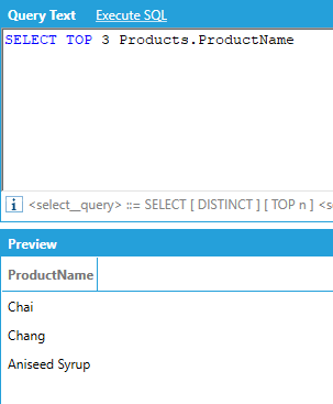
Note: The number following the TOP keyword must be a constant and cannot be an expression.
AnalytiX-BI supports the DISTINCT keyword to only return distinct rows from a query:
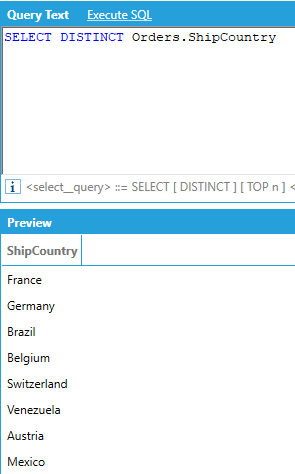
AnalytiX-BI supports the ISNULL function in the SELECT part of the query to replace NULL values occurring in the column with a default value:
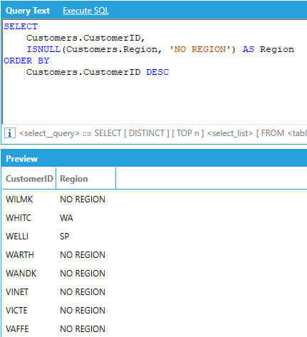
Note: the default value for the ISNULL function must be a constant and cannot be an expression or a column reference. Moreover, ISNULL cannot be used inside an aggregate function, i.e.: SUM(ISNULL(…
AnalytiX-BI supports aggregates in the SELECT attributes list. The supported aggregates are:
|
Keyword |
Description |
|
AVG |
Average |
|
MEDIAN |
Median |
|
COUNT |
Count |
|
MAX |
Maximum |
|
MIN |
Minimum |
|
SUM |
Sum |
|
STDEV |
Standard Deviation |
|
VAR |
Variance |
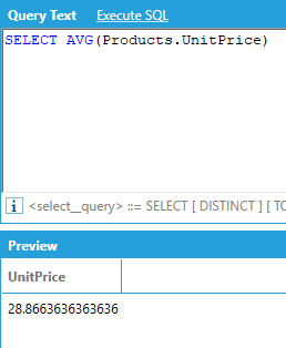
The GROUP BY keyword is not supported: results will automatically be grouped by all the attributes that do not have an a specified aggregate. For example, if we want to calculate the average unit price for all products in the Products table:
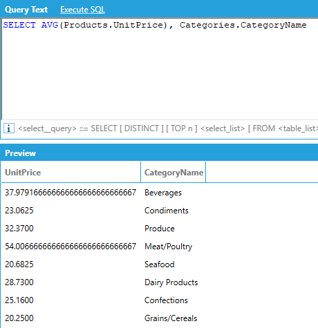
If we want to calculate the same average grouped by category name, we use the query below. The query automatically groups by CategoryName because it does not have an aggregate.
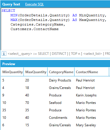
It is possible to request multiple aggregates at the same time and group by multiple attributes, even from different tables.
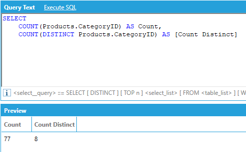
AnalytiX-BI supports calculating aggregates over only distinct values of a specific column by adding the DISTINCT qualifier before the column name inside the aggregate function, for example:
Columns of type DateTime are automatically represented as hierarchical columns by AnalytiX-BI. The level names in a DateTime hierarchy are as follows:
Year
Month
Day
Hour
Minute
Second
Hierarchical columns allow access to the levels of the hierarchy as individual columns by specifying the level name after the name of hierarchical column name, in this format [column name.level name].
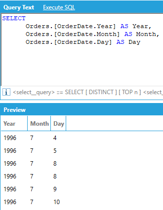
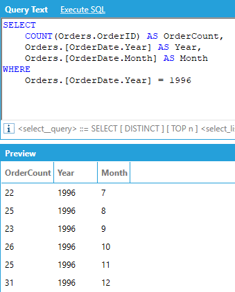
Hierarchies are extremely useful for drill-down and rollups because they allow us to aggregate and group by individual levels in the hierarchy:
In addition to DateTime columns, there are two other hierarchical columns available in AnalytiX-BI data models:
AssetPath, which is produced by the Dimensions > Assets data flow step
PointName, column produced by the Dimensions > Historical Tags
The hierarchy levels in these columns are dynamic and depend on the structure of the data imported from AssetWorX or Hyper Historian.
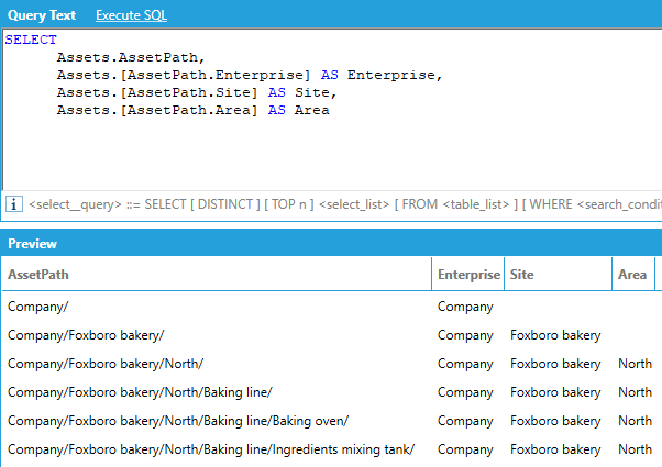
As an example, consider the following data table that we have named Assets, connected to a data flow that ingests all assets under Company in AssetWorX using a Dimensions > Assets step:
Data Table Connected to a Data Flow Ingesting Assets
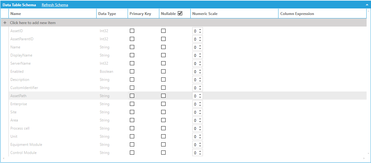
The data schema lists the AssetPath column (which is our hierarchical column) and the individual levels (Enterprise, Site, Area, etc.). Individual levels can be accessed by name in the same way as DateTime levels.
AnalytiX-BI supports column expressions, which are dynamically evaluated when the query is executed. Expressions must be enclosed in single quotes and have an alias that specifies the output column name. Any column names in the expression must be wrapped in double curly-brackets.
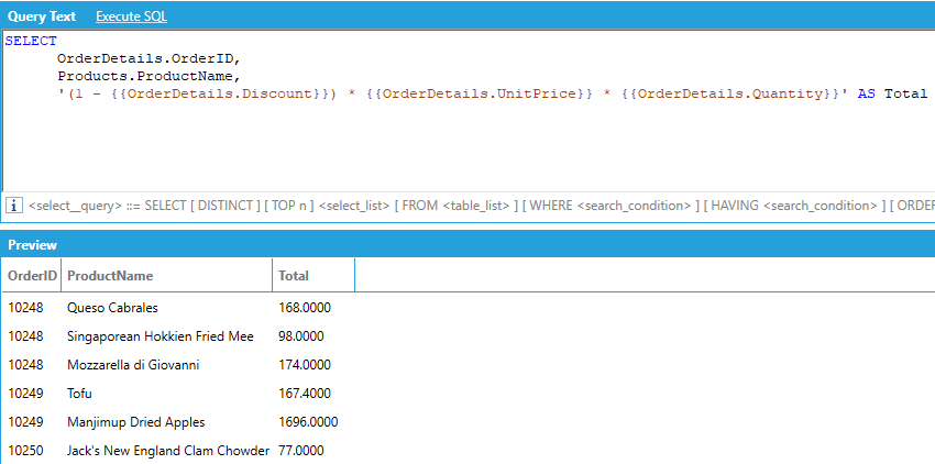
Column expressions have the same syntax as calculated columns in data tables or data flows and can reference any column in the model as a variable, even if the column is not used elsewhere in the query.
Note: It is not possible to use tabular functions like aggregates in column expressions. This is because, when evaluating column expressions, all the tables involved in the query are joined first and then the expressions are scalarly evaluated in the context of each row.
It is possible to restrict the results of an AnalytiX-BI query by adding a WHERE clause. The condition of a WHERE clause is a Boolean predicate made from one or more logical comparisons. The supported comparison operators are:
|
Operator |
Description |
|
= |
Equal |
|
<> |
Not equal (!= is also supported) |
|
> |
Greater than |
|
< |
Less than |
|
>= |
Greater than or equal |
|
<= |
Less than or equal |
|
LIKE |
String pattern matching |
|
NOT LIKE |
Negative string pattern matching |
|
IN |
Value falls into the IN list of values |
|
NOT IN |
Value does not fall into the IN list of values |
For example, we can return the name of all products for which the Category ID is 8 (Seafood):
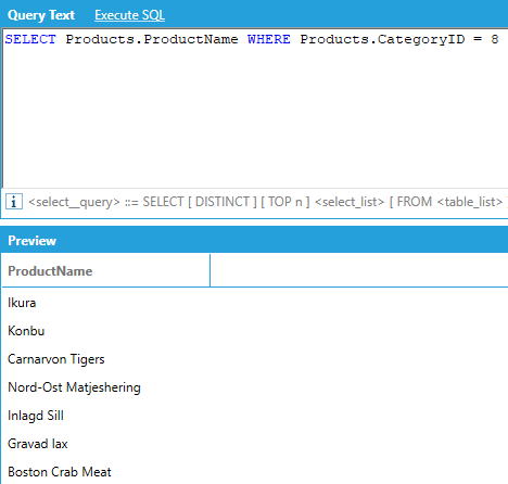
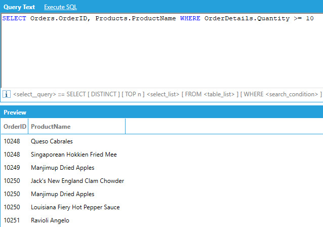
As usual, we don’t need explicit JOINs or the FROM keyword, as AnalytiX-BI can automatically compute them based on columns involved in the query.
For example, if we want to show the order ID and the product name for all orders where the quantity ordered of the product was greater than or equal to 10:
String literals must be enclosed in single quotes:
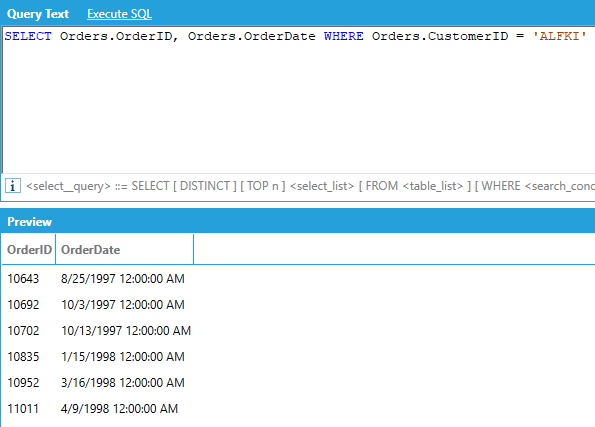
Literal single quotes and literal backslashes need to be escaped using backslash. The LIKE comparison operator uses the percent sign (%) as a wildcard, same as standard SQL. Also same as standard SQL, to match a literal percent sign, wrap it in square brackets ([%]):
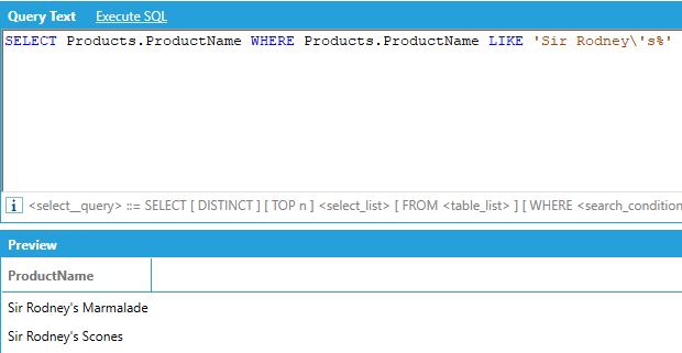
Note: It is recommended that the equals (=) or not equals (<>) operators be used whenever possible instead of LIKE. See Performance Considerations > Query Execution.
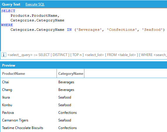
The IN operator can be used to concisely specify several values without having to OR several equality comparisons together. The set of values must be enclosed in parentheses:
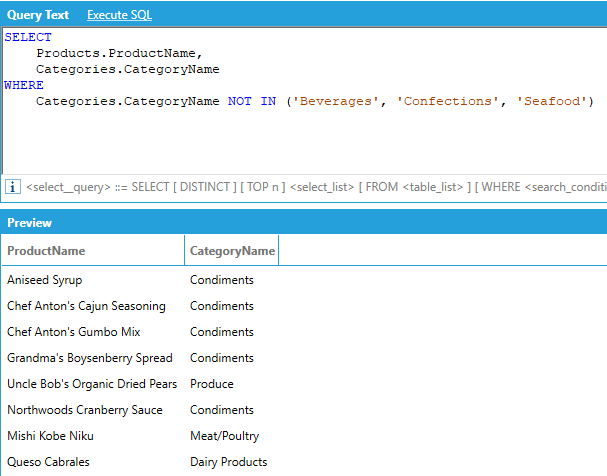
Similarly, the NOT IN operator can be used to concisely exclude several values without having to AND several inequality comparisons together:
Comparison predicates can be logically combined to form more complex predicates:
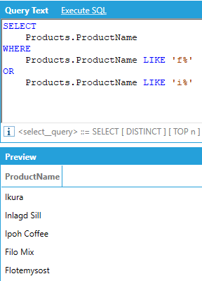
Note: Individual Boolean predicates must be comparisons between a column and a constant value. Column expressions are not supported in either side of a Boolean comparison, and it is not possible to create a predicate that compares a column with another. Also, aggregates are not supported in the WHERE clause. Instead, see the HAVING clause below.
The HAVING keyword works conceptually the same way as WHERE, but HAVING is for use with aggregates. With HAVING, the predicates are evaluated after the aggregates have been calculated, whereas the WHERE predicate is applied before calculating aggregates.
For example, let’s assume we want to return the number of orders per customer, but only for customers that have more than 20 orders:
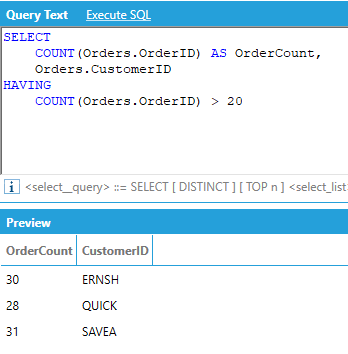
Note: Individual Boolean predicates must be comparisons between an aggregate and a constant value. Column expressions are not supported in either side of a Boolean comparison.
It is possible to sort the results of an AnalytiX-BI query using the ORDER BY clause. For example, to sort products from the most to the least expensive:
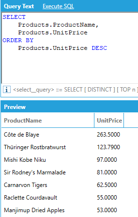
The ORDER BY clause supports the ASC and DESC modifiers to specify the order of the sorting: if no modifier is specified, ASC is used. Multiple columns can be used for sorting, and the sequence of the sort columns in the ORDER BY clause defines the organization of the sorted result set. For example:
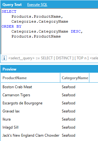
If the query contains aggregates, the result set can be sorted by aggregated values specifying the aggregate in the ORDER BY clause:
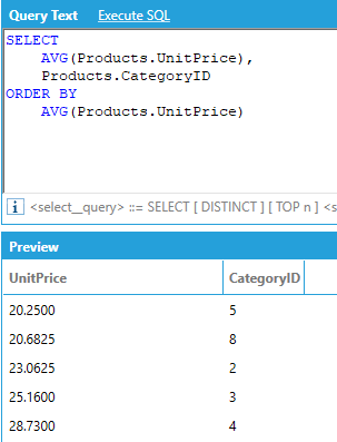
You can ORDER BY columns that are not in the SELECT clause, except when using aggregates. When using aggregates, the ORDER BY clause can only contain the attributes that are being aggregated or used as group by attributes.
AnalytiX-BI supports the PIVOT relational operator to rotate the rows of a query by turning the unique values from one column in the query into multiple columns in the output and performing aggregations where required.
For example, assume that we want to display the total of the quantities ordered for each product category per calendar year, where the categories are columns in the output:
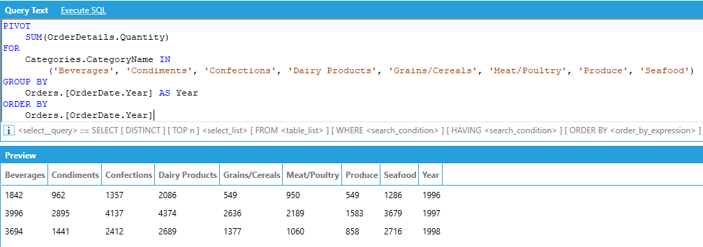
The PIVOT operator works in the following way:
We must specify the column that provides the values that will be used to fill the new pivoted columns, along with an aggregate that specifies how to combine multiple values. In our example we want to show quantity of ordered product in the transposed columns, aggregated with SUM.
We must specify the pivot column, or the column that contains the values that will be turned into columns in the output - along with the list of unique values that we want to use as columns in the output. In our example we want to use the category names as output columns of our query, and we explicitly list all the names of the categories.
Optionally, we can specify one or more attributes that will be used to group (and aggregate) the values in the output. In our example we want to SUM the quantities and group them by calendar year.
Optionally, we can specify one or more attributes to sort the output. The ORDER BY attributes must be picked from the list of attributes used in the GROUP BY list.
AnalytiX-BI automatically determines the input to the PIVOT operator by selecting the columns listed in the PIVOT query and joining the necessary tables. In our example we are using the Quantity column from the OrderDetails table, the CategoryName column from the Categories table and the OrderDate column from the Orders table. AnalytiX-BI will then build the following query as input to the PIVOT operator:
SELECT Categories.CategoryName, OrderDetails.Quantity, Orders.OrderDate FROM Categories INNER JOIN Products ON Categories.CategoryID = Products.CategoryID INNER JOIN OrderDetails ON Products.ProductID = OrderDetails.ProductID INNER JOIN Orders ON OrderDetails.OrderID = Orders.OrderID
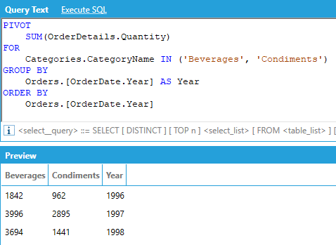
It is not necessary to specify all the unique values of the PIVOT column inside the IN. You can specify only a subset of the columns for an abbreviated result.
A number of recent enhancements have been made to the PIVOT keyword.
PIVOT queries now allow to specify GROUP BY columns either explicitly or under the PIVOT clause. For example, the following two queries are equivalent:
PIVOT
SUM(OrderDetails.Quantity),
FOR
Categories.CategoryName IN ('Beverages', 'Condiments', 'Seafood')
GROUP BY
Orders.[OrderDate.Year] AS Year
ORDER BY
Orders.[OrderDate.Year]
PIVOT
SUM(OrderDetails.Quantity),
Orders.[OrderDate.Year] AS Year
FOR
Categories.CategoryName IN ('Beverages', 'Condiments', 'Seafood')
WHERE
OrderDetails.UnitPrice > 20.0
ORDER BY
Orders.[OrderDate.Year]
Note, if GROUP BY columns are specified both in the PIVOT clause and the GROUP BY clause an error will be returned.
A WHERE clause can optionally be applied before the GROUP BY or ORDER BY clause, like follows:
PIVOT
SUM(OrderDetails.Quantity),
Orders.[OrderDate.Year] AS Year
FOR
Categories.CategoryName IN ('Beverages', 'Condiments', 'Seafood')
WHERE
OrderDetails.UnitPrice > 20.0
ORDER BY
Orders.[OrderDate.Year]
Pivoted columns can now appear in the ORDER BY clause, as in this example:
PIVOT
SUM(Products.UnitsInStock)
FOR
Categories.CategoryName IN ('Beverages', 'Condiments')
GROUP BY
Orders.[OrderDate.Year]
ORDER BY
Categories.Beverages
And PIVOT queries now allow post-filtering the pivoted dataset on pivoted columns using the HAVING statement, as in this example:
PIVOT
SUM(Products.UnitsInStock),
Orders.[OrderDate.Year]
FOR
Categories.CategoryName in ('Beverages', 'Seafood')
HAVING
Categories.Seafood > 4000
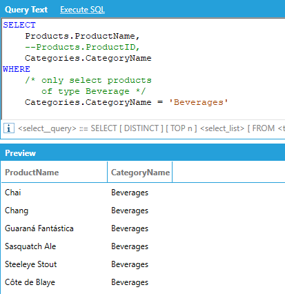
AnalytiX-BI supports comments in queries, both with the SQL single and multi-line syntax:
See Also:
Data Flows
AnalytiX-BI Server - Diagnostic Counters