Tag Properties

Tags contain the data that you are collecting and logging for trend analysis in TrendWorX64. Tags are contained in logging groups. You have control over what you call the tag data set, but the path to the OCP-UA tag is fixed to reference the particular tag of interest. In building the path to the tag, which is referred to as the signal name, you can use global and language aliasing to make it easier to create and work with tags.

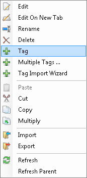
To add a tag to a logging group:

1. Right-click the logging group desired then select the Tag command from the context menu. You can also select a logging group and click Add, Tag in the edit group on the Home ribbon or use the Tag Import Wizard function.

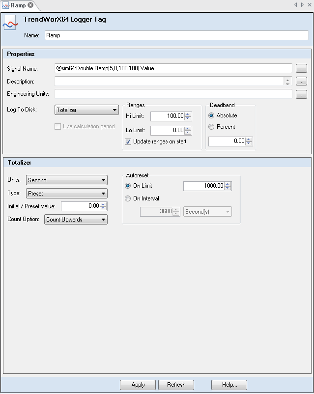
To set a tag's properties:

1. Double-click the tag or click the Edit or Edit On New Tab command in the Edit group on the Home ribbon to display the Tag property form.

   TrendWorX Tag Property Form

   

To set the data source of the tag:

• Enter the tag into the text box directly, or click the ellipsis button next to the Signal Name text box and in the Data Browser The Data Browsr refers specifically to the OPC UA tab of the Unified Data Browser. Refer to Unified Data Browser for more detail. specify the tag you wish to monitor.

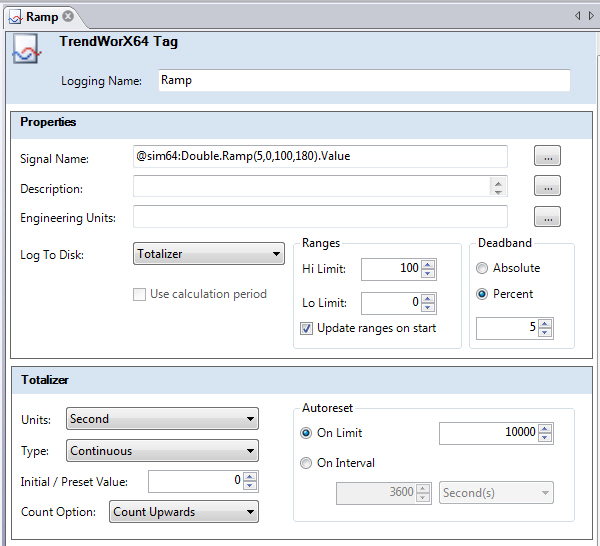
To enter a description and/or append unit names to your tag data:

• Enter any string or value you desire that is compatible with a text field into the Description and/or Engineering Units fields.

The Description and Engineering Units text boxes allow you to show information that will help you identify the tag during your work. Both are optional fields. Many of these strings are created using aliases, which you can select from the Data Browser by clicking on the respective ellipsis buttons .

Ranges and Deadband

To set the range of the samples that are collected:

• Enter the desired values into the Hi Limit and Lo Limit boxes, or enable the Update ranges on start check box to ignore the Hi Limit and Low Limit values and get the range values from the OPC UA server. Ranges from the server are updated when data logging begins.

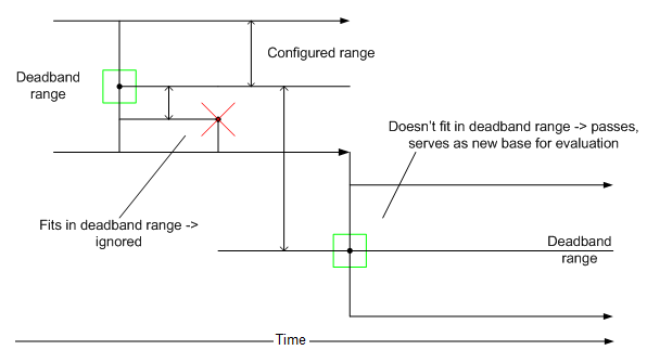
A deadband range is a range of values that surrounds a logged data point. When the logger receives another point afterward, it logs this point only if it does not lie inside of this range. This logged value then becomes the center of a new deadband range. A deadband value applies to converted analog values and is required. You can set the deadband range as an absolute value or as a percentage of the total data range.

An example of how the deadband range operates appears below.

Deadband Example

Log To Disk Function

The Log to Disk field allows you to select the value(s) of the signal that is/are logged to the database. SQL servers provide aggregate functions such as maximum/minimum, averages, and so on that you can log to disk.  If All Samples is selected, the server will log all values for that signal that were collected during the data collection period.

Aggregate functions are calculated by the database engine in one of two ways:

• Use Calculation Period Enabled: This setting forces the database engine to recalculate aggregates at sub-intervals defined in the On Interval setting within the Logging section of the Logging Group settings. To see the Logging Group settings, right-click the Logging Group within the tree and select Edit from the menu. This setting applies to Max, Min, Avg, and Std. Dev. functions only.

• Use Calculation Period Disabled: All aggregate functions are calculated when samples are written to disk and are based on all sample values collected since the previous write to disk.

The table below lists how the different following aggregate functions can be used in trends.

Aggregate Database Tag Functions

Standard Deviation is the measure of a probability distribution as a function of the spread of the group's values. It is commonly given the Greek symbol sigma (s), and is measured as the square root of the variance, or more formally the root mean square (RMS). It is calculated by finding the mean value of the population, calculating each value's deviation, squaring the deviations, finding the mean of the square and then performing a square root. For a group {1, 4, 7} the mean is 4, the deviations are {3, 0, 3}, the squares of the deviation is {9, 0, 9}, and the standard deviation would be (18/3)½ or (6)½ or approximately 2.45.

Running Aggregate Functions

Running averages are calculated over the entire data logging period using an exponentially weighted moving average (EWMA) filter equation. If the calculation period is enabled for the tag, and no new samples are received within the calculation time period, the Data Logger will use the last known value to provide a more accurate EWMA estimate. In addition, if new samples are being received irregularly, the Data Logger will try to "backfill" missing samples (by using the last known value) in order to provide a more-accurate EWMA estimate. This way the Data Logger accommodates slowly changing signals, which, due to the event nature of OPC data updates, change less frequently than the desired data collection. If the calculation period is not enabled, the Data Logger will still try to "backfill" missing samples (by using the last known value), but no new historical values will be entered to the database until a new (updated) sample arrives. The following EWMA filter equation used is:

EWMA(n) = coefficient * Measurement(n) + (1-coefficient)*EWMA(n-1)

In the equation above, n is the sample count, and coefficient is a constant typically chosen to be between 0 and 1. From this equation, we can view the EWMA estimate as a weighted average of all past and current measurements, with the coefficients of each new measurement declining geometrically. From this point of view, it is an ideal filter equation to use in the case of random individual measurements. In order to accelerate the filter convergence, the Data Logger will use the following equation:

EWMA(n) = (1/n+1) * Measurement(n) + (n/n+1)*EWMA(n-1)

Until n = 32 (i.e. using the first 32 samples). After the first 32 samples, the value of the coefficients in the EWMA equation will stay constant.

Moving Aggregate Functions

The best way to think about moving aggregate functions is to consider a moving window of samples for which the aggregate function is applied. Suppose the trend logger had a default of 4 samples in a moving window (a fourth level filter). Consider a logging session of 1 sample per second run for 60 seconds. For the first 4 values the aggregate function is applied to those values 1 through 4. In the 5th second the first sample is replaced in the moving frame by the 5th sample, and this continues for the remaining 55 seconds as each successive value replaces the signal value collected least recently.

The actual order of the moving filter is determined:

• Dynamically using the ratio of Calculation Interval/Data Collection Rate.

• Or, when there is no calculation interval used, the Logging Period/Data Collection Rate.

In instances where no sample data was collected the moving aggregate function uses the last value it calculated to fill in the necessary four signal values. Thus for a Moving Max set {4, 3, 2, 3} the max value would be 4. If the next three signals were missing, then the Moving Max set three periods later would be {3, 4, 4, 4}.

The moving aggregate function bases the quality of a calculated sample on whether there is a sample that has a "bad" quality attribute. A single bad quality sample creates an unknown aggregate result. Since the result is not entirely certain, the trend logger marks the aggregate value as bad.

Totalizer Function

When you select the Totalizer filter in the Log To Disk drop down dialog box you can create a custom filter to suit your specific needs. This Totalizer performs an integration of data values over a specified time interval. To set up the Totalizer you need to know:

1. The kind if input signals the Totalizer will be used for

2. Your expected results

3. Units of measurement for the raw data

4. Expected total values

The best application for Totalizer data is for a rate sampling:

• Totalizing a signal that comes form a flow rate gauge (liters per minute) to obtain the total number of liters that pass through the gauge during the totalizing time period.

• Totalizing the output signal of an electrical power gauge (kilowatts) to find total energy consumed during measured interval (in kilowatt-hours).

Or, some similar circumstance.

The raw signal into the Totalizer is a derivative of the value that you get with Totalizer, which integrates the samples. The totalized value should be independent of the sampling rate so that the total energy consumed in the above example is the same regardless of how often you query the power gauge. The goal of the Totalizer settings are to limit the oscillations in source values to no more than about half the sampling frequency or faster in order that the results be sufficiently accurate.

The totalized value is calculated using the trapezoidal rule for numeric integration:

S(n)=S(n-1) + 0.5 * (V(n)+V(n-1)) * (T(n)-T(n-1)) * f

where S(n) - totalized value for "current" n-th point;

S(n-1) - totalized value for "previous" (n-1)-th point;

V(n) - current raw OPC data point, T(n) - its time stamp;

V(n-1) - previous raw OPC data point, T(n-1) - its time stamp; the time stamp difference is converted to seconds; factor f provides the appropriate units conversion:

Here's an example of this calculation:

V(n=1...N) is a flow rate in liters per minute;

To get a totalized value expressed in Liters f should be (1/60)(min/sec); with the Amount per minute radio button selected.

If V(n) is sampled in Liters per seconds, f=1 with the Amount per second radio button selected.

If V(n) is sampled in Liters per hour, f=(1/3600)(hour/sec) with the Amount per hour radio button selected

The totalized value is an integral and is the total value collected for particular period expressed in proper units, which is Liters in the above examples.

The Totalizer needs to know how quickly the input signal is going to change significantly. If the value changes slowly over the course of an hour then the collection rate of a minute will suffice to get accurate results. If, on the other hand, data is changing significantly every couple of minutes, then you need to increase your data collection rate and lower the sampling interval to some number of seconds for sufficient accuracy.

If you select Totalizer from the Tag Properties dialog box, additional settings will appear.

The Totalizer offers the following parameter settings:

• Units: The Units field sets the integration constant for the totalizer filter (either Second, Minute, Hour, or Day).

• Type: The Type field sets the type of totalizer filter, which can be Continuous, Preload, or Preset.

• Initial/Preset Value: The Initial/Preset Value field sets the Initial (Pre-loaded) or Preset value based on the totalizer Type selected.

• Count Option: The Count Option field sets the integration direction of the totalizer. It can be Count Upward (from a given value) or Count Downward (to a given value).

• Auto reset: The Auto reset field sets the auto reset mode and value of the totalizer. It can be value-based or time-interval based. Once the condition is met, the totalizer will reset to the configured levels.

See also:

Tag Import Wizard

TrendWorX64 Logger