
The features on this page require a GENESIS64 Advanced license and are not available with GENESIS64 Basic SCADA .
|
|
The features on this page require a GENESIS64 Advanced license and are not available with GENESIS64 Basic SCADA . |
The AnalytiX-BI Server supports a subset of SQL for running queries against data models. Queries can be provided as part of a point name (see the "Ad Hoc Queries" section of AnalytiX-BI Runtime) or used in a data view.
In the next sections we will detail the different SQL keywords that the AnalytiX-BI server’s query engine supports, and how they may differ from standard SQL.
SELECT
Using SELECT to retrieve rows and columns
Automatically generated aliases
Using SELECT with calculations and scalar functions
Using SELECT with DISTINCT
Using SELECT with TOP
FROM
JOIN
GROUP BY
WHERE
Equals
Not Equals
Greater Than
Greater Than or Equal
Less Than
Less Than or Equal
[NOT] LIKE
[NOT] BETWEEN
IS [NOT] NULL
[NOT] IN
[NOT] EXISTS
HAVING
ORDER BY
OFFSET
FETCH
Aggregate Functions
AVG
COUNT
MAX
MIN
MEDIAN
STDEV
SUM
VAR
UNION [ALL]
COLLATE
CASE
Simple CASE
Searched CASE
Hierarchical Columns
PIVOT
Comments
In AnalytiX-BI, each column, expression and parameter has an associated data type, which specifies what kind of data the attribute can hold. When two expressions that have different data types are combined by an operator or a function, the characteristics of the result are determined by the data type precedence rules.
The following table describes all the data types supported by AnalytiX-BI, in increasing order of precedence (i.e.: the first type in the list has the lowest precedence, while the last type in the list has the highest precedence).
|
Data type |
Description |
|
String |
Unicode character string, with no maximum length. |
|
Guid |
A 128-bit (16 bytes) unique identifier |
|
Boolean |
A Boolean (true or false) value |
|
Byte |
An 8-bit unsigned integer. Range is from 0 through positive 255 |
|
SByte |
An 8-bit signed integer. Range is from negative 128 through positive 127 |
|
Int16 |
A 16-bit signed integer. Range is from negative 32,768 through positive 32,767 |
|
Uint16 |
A 16-bit unsigned integer. Range is from 0 through 65,535 |
|
Int32 |
A 32-bit signed integer. Range is from negative 2,147,483,648 through positive 2,147,483,647 |
|
Uint32 |
A 32-bit unsigned integer. Range is from 0 through 4,294,967,295 |
|
Single |
A 64-bit signed integer. Range is from negative 9,223,372,036,854,775,808 through positive 9,223,372,036,854,775,807 |
|
Double |
A double-precision 64-bit number with values ranging from negative 1.79769313486232e308 to positive 1.79769313486232e308, as well as positive or negative zero, PositiveInfinity, NegativeInfinity, and not a number (NaN) |
|
Decimal |
A 12 bytes decimal numbers ranging from positive 79,228,162,514,264,337,593,543,950,335 to negative 79,228,162,514,264,337,593,543,950,335 |
|
TimeSpan |
A time interval (duration of time or elapsed time) that is measured as a positive or negative number of days, hours, minutes, seconds, and fractions of a second |
|
DateTime |
Represents dates and times with values ranging from 00:00:00 (midnight), January 1, 0001 Anno Domini (Common Era) through 11:59:59 P.M., December 31, 9999 A.D. (C.E.) in the Gregorian calendar. |
|
DateTimeOffset |
Represents a point in time, typically expressed as a date and time of day, relative to Coordinated Universal Time (UTC) |
When an operator combines expressions of different data types, the type with the lower precedence is first converted to the data type with the higher precedence. For operators combining operand expressions having the same data type, the result of the operation has that data type.
Implicit conversion is supported from any type to a higher precedence type, with the exception of GUID which cannot be implicitly converted to other types. For more information on type conversions, consult the CAST and CONVERT functions.
The following query uses implicit conversion to convert the literal 1 into the equivalent integer. The conversion happens because string has a lower precedence than Int32 and so it gets converted.
SELECT * FROM Products WHERE ProductID = '1'
With the evolution of the AnalytiX-BI SQL language, some of the features from the previous version are being deprecated and kept for backwards-compatibility reasons only. For this reason, AnalytiX-BI introduces the concept of Compatibility Level for Data Models, which determines how some of the features of the SQL language work.
Currently, Data Models belonging to a configuration that has been upgraded from a previous version (prior to 10.97.1) will be set at compatibility level 0x109700 and function in backwards-compatibility mode. Data Models created in the current version will be set at compatibility level 0x109710 and will disable the backwards-compatible features.
Note: The Data Model compatibility level is currently not displayed in the UI.
The differences between compatibility and “normal” mode are the following:
Aggregated columns without an explicit alias will produce a different auto-generated output column name when running in “normal” mode. See Automatically generated aliases for more information.
Expressions written with the Expression Engine syntax as string literals will be parsed and executed only when running in backwards-compatibility mode. See Using SELECT with calculations and scalar functions for more information.
Retrieves data from a data model and enables the selection of one or many rows or columns from one or many tables.
SELECT needs to be followed by a list of attributes. Table or column identifiers containing reserved symbols (such as spaces, commas, or periods) must be enclosed in square brackets.
The following example returns all rows and all columns from the Orders table in the default Northwind data model. All columns are returned using the * (star) qualifier.
SELECT * FROM Orders
Column names can be explicitly listed after the SELECT keyword to retrieve a subset of the columns. Projected columns can also be renamed using the AS keyword.
SELECT OrderID AS ID, CustomerID, OrderDate FROM Orders
Projected columns that are not aliased will produce an output column with the same name as the column itself. The following query will produce two output columns named CategoryID and CategoryName.
SELECT CategoryID, CategoryName FROM Categories
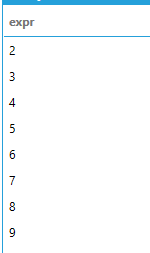
If an expression is used without an alias, the resulting output column will be named expr{n}, where n is a three-digit integer. The following query will produce one output column named expr000.
SELECT CategoryID + 1 FROM Categories
Aggregated columns without an alias will also produce output columns named expr{n}. The following query will produce two output columns named expr000 and expr001.
SELECT MAX(UnitPrice), MIN(UnitPrice) FROM Products
Backwards compatibility: This behavior is different for data models that function at compatibility level of 0x109700 (backwards-compatible). For these models, aggregated columns with no alias will produce output columns named as {aggregated column name}[_n] where aggregated column name is the name of the column being aggregated, optionally followed by an integer qualifier to make output column names unique.
The following query will produce one output column named UnitPrice.
SELECT MAX(UnitPrice) FROM Products
The following query will instead produce two output columns named UnitPrice and UnitPrice_1.
SELECT MAX(UnitPrice), MIN(UnitPrice) FROM Products
Expressions and scalar functions can be used in the SELECT list to perform calculations. The next example calculates the total price for each product in an order:
SELECT OrderID, ProductID, UnitPrice * Quantity * (1 - Discount) AS TotalPrice
FROM [OrderDetails]
Expressions can generally be used anywhere where a column reference can be used, with the exception of the ON clause in JOIN predicate where only column references can be used.
Besides arithmetic operators, AnalytiX-BI supports an extensive list of functions that can be used in expressions. For more information refer to the Scalar Functions section.
Backwards compatibility: Previous versions of AnalytiX-BI only allowed expressions in the SELECT list, and required the expressions to be written:
As string literals
With a mandatory alias
Referencing columns using the Expressions Engine’s variable syntax with double curly braces
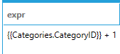
The following query illustrates how such expressions work in data models at compatibility level of 0x109700 (backwards-compatible).
SELECT '{{Categories.CategoryID}} + 1' AS expr
This query produces the following result set:
When a data model is at compatibility level of 0x109710 (current) string literals will not be parsed as expressions, but simply returned as literals. The previous query, in this case, will produce a one column, one row result set containing the literal string:
It is still possible to use the Expression Engine syntax for data models at compatibility level 0x109710 by enclosing the literal string expression with the EXPRESSION keyword. The following query parses and executes the expression and produces the same result as the query without the EXPRESSION keyword at compatibility level 0x109700.
SELECT EXPRESSION('{{Categories.CategoryID}} + 1') AS expr
The DISTINCT keyword can be used to retrieve unique rows only from the results of a query. The following example retrieves all the unique titles from the Customers table.
SELECT DISTINCT ContactTitle FROM Customers
The TOP keyword limits the number of rows returned by a query to a specified number of rows. Percentages are not supported by AnalytiX-BI. The following example retrieves the top 10 products with highest unit price.
SELECT TOP 10 * FROM Products
ORDER BY UnitPrice DESC
The FROM keyword is generally required in AnalytiX-BI queries, unless the query is selecting only constants.
Tables specified with the FROM keyword can be aliased for self-joining purposes or just to simplify the query. The following example shows how to retrieve columns from a couple of joined tables using aliases.
SELECT c.CategoryName, p.ProductName
FROM Categories AS c INNER JOIN Products AS p
ON c.CategoryID = p.CategoryID
Note: the AS keyword is required in AnalytiX-BI.
The argument to the FROM keyword can be either a table, a view, a parameterized view or a subquery. The following example shows how to retrieve data from a parameterized view that returns orders given a customer ID.
SELECT * FROM OrdersByCustomerID('ALFKI')
The following example shows how to use a subquery in the FROM clause. Note that the subquery requires an alias using the AS keyword in order to qualify the columns projected by the subquery.
SELECT t.CustomerID, t.OrderID
FROM
(SELECT c.CustomerID, o.OrderID, o.OrderDate
FROM Customers AS c INNER JOIN Orders AS o
ON c.CustomerID = o.CustomerID
WHERE o.OrderDate > '1/1/1997') AS t
ORDER BY t.OrderDate
AnalytiX-BI allows omitting the FROM keyword and the table(s) involved in the query are automatically determined from the list of requested attributes. When omitting the FROM keyword it is required that all attributes used in the query are fully qualified with their table name, as shown in the following example.
SELECT Categories.CategoryID, Categories.CategoryName
Note: although this syntax is supported for backwards compatibility, it is recommended to always specify the table(s) involved in the query using the FROM keyword.
A joined table is a result set that is the product of two or more tables. AnalytiX-BI supports INNER, LEFT OUTER and RIGHT OUTER joins.
The following query retrieves the quantity of products for each order using an inner join.
SELECT OrderID, ProductName, Quantity
FROM Products AS p INNER JOIN OrderDetails AS od
ON p.ProductID = od.ProductID
Note: selected columns do not have to be qualified when their name is unique among the joined tables.
The following example shows a query that uses a LEFT join to display the list of customers without any associated orders.
SELECT ContactName, OrderID
FROM Customers AS c LEFT JOIN Orders AS o
ON c.CustomerID = o.CustomerID
WHERE o.OrderID IS NULL
ORDER BY c.ContactName
Similarly, the following query uses a RIGHT join to display all order numbers that do not have a customer associated with them.
SELECT ContactName, OrderID
FROM Customers AS c RIGHT JOIN Orders AS o
ON c.CustomerID = o.CustomerID
WHERE c.ContactName IS NULL
ORDER BY o.OrderID
If relationships between tables are established in the data model, the JOIN keyword can be omitted, however all columns in the query must be fully qualified. AnalytiX-BI will determine the join path among all the tables that are referenced in the query automatically. The following query calculates the total for each order without having to specify explicit the FROM or JOIN keywords for the Orders and OrderDetails tables.
SELECT Orders.CustomerID, Orders.OrderDate, SUM(OrderDetails.UnitPrice * OrderDetails.Quantity * (1 - OrderDetails.Discount)) AS OrderTotal
ORDER BY Orders.OrderDate
AnalytiX-BI automatically determines the join path between the Orders and OrderDetails table based on the relationships configured in the model.
Note: when the FROM and JOIN keywords are omitted, AnalytiX-BI automatically performs INNER joins.
Note: although this syntax is supported for backwards compatibility, it is recommended to always specify the tables involved in the query using the FROM keyword and explicitly define the desired joins using the JOIN keyword.
Divides the query results into groups of rows, usually for the purpose of performing one or more aggregations on each group. The SELECT statement returns one row per group. The arguments to GROUP BY must be one or more columns or non-aggregate expressions.
The following example calculates the total for all orders per calendar year.
SELECT SUM(Quantity * UnitPrice * (1 - Discount)) AS Total, year(OrderDate) AS Year
FROM OrderDetails AS od INNER JOIN Orders AS o
ON od.OrderID = o.OrderID
GROUP BY year(OrderDate)
When aggregate functions are used in the SELECT the GROUP BY keyword can be omitted: in this case AnalytiX-BI will automatically group by all the columns specified in the SELECT that do not have an aggregate function specified.
The following query calculates the average unit price for each category.
SELECT AVG(UnitPrice), CategoryName
FROM Products AS p INNER JOIN Categories AS c
ON p.CategoryID = c.CategoryID
This notation requires projecting all the columns for which we want to group by: in order to group by a column that is not projected the GROUP BY keyword is required.
Note: although this syntax is supported for backwards compatibility, it is recommended to always specify the GROUP BY keyword in order to explicitly define the group by columns.
It is possible to restrict the results of an AnalytiX-BI query by adding a WHERE clause. The condition of a WHERE clause is a Boolean predicate made from one or more logical comparisons. Comparisons are allowed generically between columns and/or expressions.
The following query retrieves all products that are discontinued by comparing a column to a constant.
SELECT * FROM Products WHERE Discontinued = true
The following query retrieves all products that have to be reordered and are not discontinued, performing a comparison between two columns.
SELECT * FROM Products WHERE UnitsInStock <= ReorderLevel AND Discontinued = false
Predicates can also use generic expressions. The following query retrieves all orders that have been placed in August 1997 by using the year and month functions.
SELECT * FROM Orders WHERE year(OrderDate) = 1997 AND month(OrderDate) = 8
Below is the list of the supported comparison operators for search predicates.
Tests equality between two expressions. The following query retrieves all the products that have their CategoryID equal to 8.
SELECT * FROM Products WHERE UnitPrice = 8
Tests inequality between two expressions. The following query retrieves all the products that have their CategoryID not equal to 3.
SELECT * FROM Products WHERE UnitPrice <> 3
Tests inequality between two expressions. The following query retrieves all the products that have their CategoryID not equal to 5.
SELECT * FROM Products WHERE UnitPrice != 40
Tests whether the left expression is greater than the right expression. The following query retrieves all products that have a UnitPrice greater than 40.
SELECT * FROM Products WHERE UnitPrice > 40
Tests whether the left expression is greater than or equal to the right expression. The following query retrieves all products that have a UnitPrice greater than or equal to 40.
SELECT * FROM Products WHERE UnitPrice >= 40
Tests whether the left expression is less than the right expression. The following query retrieves all products that have a UnitPrice less than 40.
SELECT * FROM Products WHERE UnitPrice < 40
Tests whether the left expression is less than or equal to the right expression. The following query retrieves all products that have a UnitPrice less than or equal to 40.
SELECT * FROM Products WHERE UnitPrice <= 40
Indicates that the character string on the right is to be used with pattern matching against the left expressions.
The % (percent) character can be used as a wildcard to match any string of zero or more characters. The following query retrieves all customers whose ContactName starts with a and ends with o.
SELECT ContactName FROM Customers WHERE ContactName LIKE 'a%o'
The _ (underscore) character can be used as a wildcard to match any single character. The following query retrieves all customers whose CustomerID starts with TRA and ends with H.
SELECT * FROM Customers WHERE CustomerID LIKE 'TRA_H'
Square brackets can be used to match any single character enclosed in the brackets. The following query retrieves all customers whose CustomerID starts with B and has a second letter either a L or an O.
SELECT * FROM Customers WHERE CustomerID LIKE 'B[LO]%'
The ^ (caret) character can be used with square brackets in order to match any characters not enclosed in the brackets. The following query retrieves all customers whose CustomerID starts with B and has a second letter that is not L or S.
SELECT * FROM Customers WHERE CustomerID LIKE 'B[^LS]%'
Prefixing the LIKE keyword with NOT produces the negation of the result. The following query retrieves all customers whose CustomerID does not start with A.
SELECT * FROM Customers WHERE CustomerID NOT LIKE 'A%'
To match a literal % (percent) or _ (underscore) characters they must be enclosed in square brackets. The following query retrieves all bikes from a hypothetical Bikes table that have their discount set to 30%.
SELECT * FROM Bikes WHERE Discount LIKE '30[%]'
Tests whether the value of an expression is between two other expressions. The following query retrieves all orders places between two specific dates.
SELECT * FROM Orders WHERE OrderDate BETWEEN '1997-09-03' AND '1997-09-05'
Bounds are included in the result. Prefixing the BETWEEN keyword with NOT returns all rows not in the specified interval, not including the bounds. The following query retrieves all orders not placed between two specific dates and made in September 1997.
SELECT * FROM Orders
WHERE OrderDate NOT BETWEEN '1997-09-10' AND '1997-09-20'
AND year(OrderDate) = 1997
AND month(OrderDate) = 9
Tests whether the left expression is NULL. The following query retrieves all customers whose fax number is NULL.
SELECT * FROM Customers WHERE Fax IS NULL
Test whether the left expression is included or excluded from a list; the list can be a set of constants, column references, expressions or a subquery. The following query retrieves all products that have a CategoryID of either 1 or 2.
SELECT * FROM Products WHERE CategoryID IN (1, 2)
When using a subquery, the subquery must return a single column of a type that is compatible with the type on the column on the left of the IN. The following query retrieves the company name for all customers who have placed an in September 1996.
SELECT CompanyName FROM Customers WHERE CustomerID IN (SELECT CustomerID FROM Orders WHERE OrderDate BETWEEN '9/1/96' AND '9/30/96')
Used with a subquery to test for existence (or non-existence) of rows returned by the subquery. When testing for existence, the values in the rows returned from the subquery are irrelevant, as EXISTS only needs to check for the existence of returned rows. For this reason, the subqueries written with EXISTS are typically in the form of SELECT * or SELECT 1.
The following query produces the same output as the query in the previous section, using EXISTS instead of IN.
SELECT CompanyName FROM Customers AS c WHERE EXISTS (SELECT 1 FROM Orders WHERE c.CustomerID = CustomerID AND OrderDate BETWEEN '9/1/96' AND '9/5/96')
NOT EXISTS can be used to test for absence of rows returned from the subquery, and is generally preferable to NOT IN. The following query retrieves all customers that have not placed an order.
SELECT CustomerID FROM Customers AS c WHERE NOT EXISTS (SELECT 1 FROM Orders WHERE c.CustomerID = Orders.CustomerID)
The HAVING keyword works conceptually the same way as WHERE, but HAVING specifies a search condition for a group or an aggregate.
Note: with HAVING, the predicates are evaluated after the aggregates have been calculated, whereas the WHERE predicate is applied before calculating aggregates.
The following query returns only customers that have placed more than twenty orders.
SELECT CustomerID, COUNT(OrderID) FROM Orders GROUP BY CustomerID HAVING COUNT(OrderID) > 20
ORDER
Orders the result set of a query by the specified column list and, optionally, limit the rows returned to a specified range. It is possible to ORDER BY columns that are not in the SELECT clause, except when using aggregates. When using aggregates, the ORDER BY clause can only contain the attributes that are being aggregated or used as group by attributes.
Note: the order in which the rows are returned from a query is not guaranteed unless ORDER BY is used.
The following query retrieves the list of products ordered from the most expensive to the least expensive.
SELECT ProductName, UnitPrice FROM Products ORDER BY UnitPrice DESC
The ORDER BY clause supports the ASC and DESC modifiers to specify the order of the sorting: if no modifier is specified, ASC is used. Multiple columns can be used for sorting, and the sequence of the sort columns in the ORDER BY clause defines the organization of the sorted result set. The following query orders products by category name first and then by product name.
SELECT CategoryName, ProductName
FROM Categories AS c INNER JOIN Products AS p ON c.CategoryID = p.CategoryID
ORDER BY CategoryName, ProductName
The columns in the ORDER BY can be column references or expressions. The following query retrieves the month total for all orders placed in 1997, ordered by month.
SELECT SUM(Quantity * UnitPrice * (1 - Discount)) AS Total, month(OrderDate) AS Month
FROM OrderDetails AS od INNER JOIN Orders AS o ON od.OrderID = o.OrderID
WHERE year(OrderDate) = 1997
GROUP BY month(OrderDate)
ORDER BY month(OrderDate)
ORDER BY can also reference columns appearing in the SELECT list by their alias. The following query orders categories by their average product unit price.
SELECT CategoryName, AVG(UnitPrice) AS AvgUnitPrice
FROM Categories AS c INNER JOIN Products AS p ON c.CategoryID = p.CategoryID
GROUP BY CategoryName
ORDER BY AvgUnitPrice
Specifies the number of rows to skip before starting to return rows from the query. This value must be an integer constant greater or equal to zero. The following query returns rows from the Products table, skipping the first 30 rows.
SELECT * FROM Products ORDER BY ProductID OFFSET 30
Specifies the number of rows to return after the OFFSET clause has been processed. The value must be an integer constant greater or equal to zero. The following query skips the first ten rows from the Products table and returns the next fifteen rows.
SELECT * FROM Products ORDER BY ProductID OFFSET 10 FETCH 15
An aggregate function performs a calculation on a set of values and returns a single value. Values can be divided into groups using the GROUP BY keyword, and aggregate functions will be calculated individually per group; when no GROUP BY expressions are specified, the whole input is treated as a single group. The argument to an aggregate function can be a column reference or an expression.
With the exception of COUNT(*) all aggregate functions ignore NULL values. If an aggregate function is applied to all NULL values, its result will be NULL with the exception of COUNT – where the result will be 0 – and COUNT(*), where the result will be the number of rows.
Aggregate functions also support the DISTINCT keyword: when used, the aggregate function will be applied only to distinct values.
Returns the sum of all the values, or only the DISTINCT values, in the expression. SUM can only be used with numeric columns. NULL values are ignored. The following query returns the average unit price of all products by category.
SELECT AVG(UnitPrice) AS [Average Price], CategoryName
FROM Products AS p INNER JOIN Categories AS c ON p.CategoryID = c.CategoryID
GROUP BY CategoryName
Returns the count of all the values, or only the DISTINCT values, in the expression. COUNT can be used with columns of any type and the return type is always integer. NULL values are ignored. The following query returns the number of orders placed by individual customers in 1997.
SELECT COUNT(OrderID) AS OrdersCount, CustomerID FROM Orders
WHERE year(OrderDate) = 1997
GROUP BY CustomerID
The following query returns the count of all distinct customer titles.
SELECT COUNT(DISTINCT ContactTitle) AS Title FROM Customers
When COUNT(*) is used, it specified that COUNT should count all rows, including duplicate rows or rows that contain null values. COUNT(*) does not take an input expression to indicate that it does not use information about any particular column during the calculation. DISTINCT cannot be used with COUNT(*). The following query returns the total number of items in the Products table.
SELECT COUNT(*) FROM Products
Returns the maximum of all the values in the expression. MAX can be used with numeric, date time and string columns. NULL values are ignored. The following query returns the highest unit price for all products.
SELECT MAX(UnitPrice) FROM Products
Returns the minimum of all the values in the expression. MIN can be used with numeric, date time and string columns. NULL values are ignored. The following query returns the lowest unit price for all products.
SELECT MIN(UnitPrice) FROM Products
Returns the median of all the values, or only the DISTINCT values in the expression. MEDIAN can be used with numeric columns only. NULL values are ignored. The following query returns the median unit price for all products by category.
SELECT MEDIAN(UnitPrice) AS [Median Price], CategoryName
FROM Products AS p INNER JOIN Categories AS c ON p.CategoryID = c.CategoryID
GROUP BY CategoryName
Returns the statistical standard deviation of all the values, or only the DISTINCT values, in the expression. STDEV can only be used with numeric columns. NULL values are ignored. The following query returns the statistical standard deviation for product unit prices by category.
SELECT STDEV(UnitPrice) AS [Price Standard Deviation], CategoryName
FROM Products AS p INNER JOIN Categories AS c ON p.CategoryID = c.CategoryID
GROUP BY CategoryName
Returns the sum of all the values, or only the DISTINCT values, in the expression. SUM can only be used with numeric columns. NULL values are ignored. The following query returns the total of all orders grouped by calendar year.
SELECT SUM(Quantity * UnitPrice * (1 - Discount)) AS Total, year(OrderDate) AS Year
FROM OrderDetails AS od INNER JOIN Orders AS o
ON od.OrderID = o.OrderID
GROUP BY year(OrderDate)
Returns the statistical variance of all the values, or only the DISTINCT values, in the expression. STDEV can only be used with numeric columns. NULL values are ignored. The following query returns the statistical variance for product unit prices by category.
SELECT VAR(UnitPrice) AS [Price Variance], CategoryName
FROM Products AS p INNER JOIN Categories AS c ON p.CategoryID = c.CategoryID
GROUP BY CategoryName
Concatenates the result sets of two queries into a single result set. In order to union the result sets, the two queries must:
Return the same number of columns, in the same order
The data types for the columns at the same position in the two results sets must be the same
When using UNION ALL the result set is allowed to contain duplicate rows, so it will contain all rows from both sets. When using UNION duplicate rows will be removed. The following query returns the union of customers and employees.
SELECT ContactName, CompanyName FROM Customers
UNION ALL
SELECT FirstName + ' ' + LastName, 'Northwind' FROM Employees
The order of the rows in the output is generally unspecified. To apply a specific order, the ORDER BY keyword can be used outside the union. The following query returns the union of customers and employees, ordered by ContactName.
SELECT * FROM
(SELECT ContactName, CompanyName FROM Customers
UNION ALL
SELECT FirstName + ' ' + LastName, 'Northwind' FROM Employees) AS t
ORDER BY ContactName
Represents a collation cast operation when applied to character string expression. AnalytiX-BI collations are composed by two parts, separated by underscore:
A culture identifier, which follows the .NET rules for culture identifiers. The name is a combination of an ISO 693 two-letter culture code associated with a language and an ISO 3166 two-letter subculture code associated with a country or region. Examples include jp-JP for Japanese (Japan) and en-US for English (United States). For more information refer to Culture names and Identifiers for .NET.
A case identifier, which can be one of the two possibilities:
ci – which stands for case-insensitive
cs – which stands for case-sensitive
AnalytiX-BI sets the collation for all string columns in a data model to the system’s current culture, case-insensitive. This means that string comparisons will follow the lexical rules of the system’s culture and will be case-insensitive.
Note: It is currently not possible to configure the default collation for a data model or an individual string column.
The following query will return the row associated with the Beverages categories because the default collation is case-insensitive.
SELECT * FROM Categories WHERE CategoryName = 'beverages'
The following query will not return any row because it is forcing a case-sensitive comparison using the COLLATE keyword.
SELECT * FROM Categories WHERE CategoryName COLLATE en-us_cs = 'beverages'
The COLLATE keyword can be used after column references of type string or after string literals.
Evaluates a list of conditions and returns one of multiple possible result expressions. The CASE expression has two formats:
Simple CASE, which compares an expression to a set of simple expressions to determine the result
Searched CASE, in which a set of Boolean expressions are evaluated to determine the result
CASE can be used in anywhere an expression can be used, like in a SELECT list, in a WHERE statement, ORDER BY, etc.
The simple CASE expression operates by sequentially comparing the first expression to the expression in each WHEN clause for equivalency. If the expressions are equivalent, the expression in the THEN clause will be returned.
Simple CASE supports an optional ELSE clause which allows to specify a default value to return if none of the expressions in the WHEN clauses is equivalent to the first expressions. When the ELSE clause is not provided, NULL is returned when none of the expressions in the WHEN clauses is equivalent to the first expression.
The following query returns all products with a string description on whether the product has been discontinued or not. In this example the first expression (the column Discontinued) gets compared with the Boolean values false and then true in order to produce the result in the THEN clause.
SELECT ProductName,
CASE Discontinued
WHEN false THEN 'Available'
WHEN true THEN 'Discontinued'
END AS Status
FROM Products
The following query uses the ELSE clause to return a UnitPrice discounted by 10% for all beverages, a UnitPrice increased by 5% for all seafood and an unmodified UnitPrice for any other product type.
SELECT ProductName, UnitPrice,
CASE CategoryID
WHEN 1 THEN UnitPrice * 0.90
WHEN 8 THEN UnitPrice * 1.05
ELSE UnitPrice
END AS ModifiedUnitPrice
FROM Products
The searched CASE expression operates by sequentially evaluating the Boolean expressions in each WHEN clause. If an expression evaluates to true, the expression in the THEN clause is returned.
Searched CASE supports an optional ELSE clause which allows to specify a default value to return if none of the expressions in the WHEN clauses evaluate to true. When the ELSE clause is not provided, NULL is returned when none of the expressions in the WHEN clauses evaluate to true.
The following query returns the fax number for all customers and defaults to the string No Fax for customer that do not have a fax number.
SELECT ContactName,
CASE
WHEN Fax IS NULL THEN 'No Fax'
ELSE Fax
END
FROM Customers
Columns of type DateTime are automatically represented as hierarchical columns by AnalytiX-BI. The level names in a DateTime hierarchy are as follows:
Year
Month
Day
Hour
Minute
Second
Hierarchical columns allow access to the levels of the hierarchy as individual columns by specifying the level name after the name of hierarchical column name. The following query retrieves the year, month and day parts of the OrderDate column.
SELECT
Orders.[OrderDate.Year] AS Year,
Orders.[OrderDate.Month] AS Month,
Orders.[OrderDate.Day] AS Day
Note: When referencing a hierarchy level, the column must always be fully qualified with the table name; the column name is followed by a period and then the level name, and they both have to be enclosed in square brackets.
The hierarchical access, although supported at all compatibility levels, should only be used for backwards-compatibility. In the current version of AnalytiX-BI the preferred way of retrieving individual levels of a DateTime hierarchy is to use either the DATEPART function, or the individual functions to extract parts of a date and time.
The following query retrieves the same information as the previous query using the DATEPART function.
SELECT
DATEPART(OrderDate, 'year') AS Year,
DATEPART(OrderDate, 'month') AS Month,
DATEPART(OrderDate, 'day') AS Day
FROM Orders
Alternatively, the individual functions can be used to obtain the same result.
SELECT
year(OrderDate) AS Year,
month(OrderDate) AS Month,
day(OrderDate) AS Day
FROM Orders
For more information about the individual functions please refer to Date and Time functions.
In addition to DateTime columns, there are two other hierarchical columns available in AnalytiX-BI data models:
AssetPath, which is produced by the Dimensions > Assets data flow step
PointName, column produced by the Dimensions > Historical Tags
The hierarchy levels in these columns are dynamic and depend on the structure of the data imported from AssetWorX or Hyper Historian.
As an example, consider the following data table that we have named Assets, connected to a data flow that ingests all assets under Company in AssetWorX using a Dimensions > Assets step:
Data Table Connected to a Data Flow Ingesting Assets
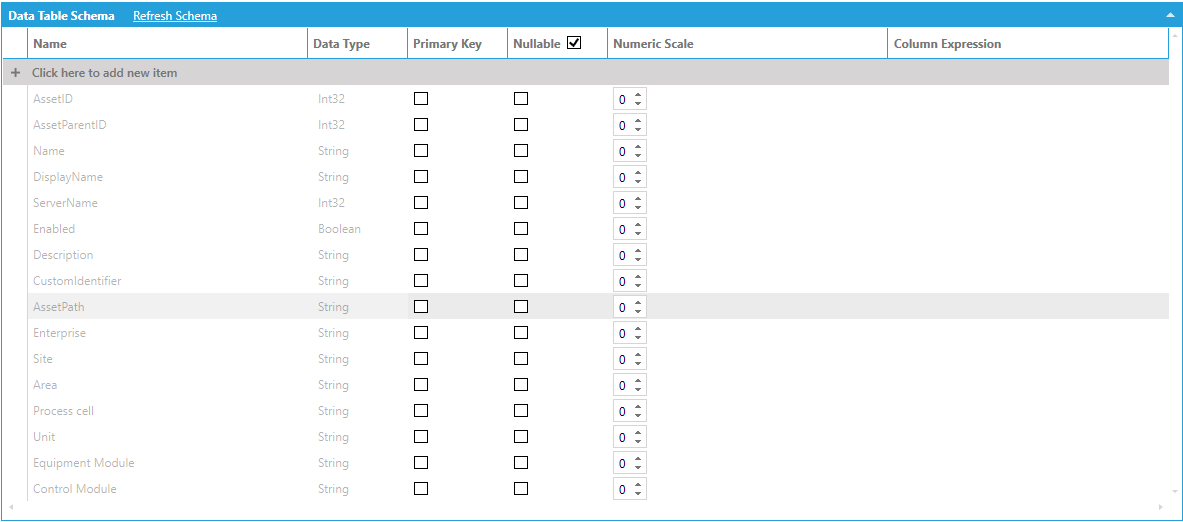
The data schema lists the AssetPath column (which is our hierarchical column) and the individual levels (Enterprise, Site, Area, etc.). Individual levels can be accessed by name in the same way as DateTime levels.
The following query selects the AssetPath column, along with the Enterprise, Site and Area levels.
SELECT
Assets.AssetPath,
Assets.[AssetPath.Enterprise] AS Enterprise,
Assets.[AssetPath.Site] AS Site,
Assets.[AssetPath.Area] AS Area
As in the case with the DateTime dimension, hierarchical access should only be used for backwards-compatibility. The current version of AnalytiX-BI, unlike previous versions, also exposes the level columns as individual columns in the table.
The following query retrieves the same data as the previous query by referencing the level columns directly without the need of hierarchical access.
SELECT
AssetPath,
Enterprise,
Site,
Area
FROM Assets
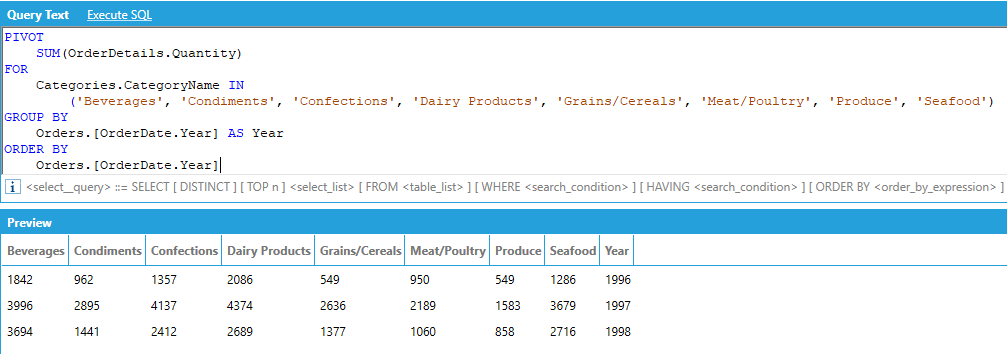
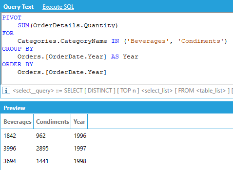
AnalytiX-BI supports the PIVOT relational operator to rotate the rows of a query by turning the unique values from one column in the query into multiple columns in the output and performing aggregations where required.
For example, assume that we want to display the total of the quantities ordered for each product category per calendar year, where the categories are columns in the output:
The PIVOT operator works in the following way:
We must specify the column that provides the values that will be used to fill the new pivoted columns, along with an aggregate that specifies how to combine multiple values. In our example we want to show quantity of ordered product in the transposed columns, aggregated with SUM.
We must specify the pivot column, or the column that contains the values that will be turned into columns in the output - along with the list of unique values that we want to use as columns in the output. In our example we want to use the category names as output columns of our query, and we explicitly list all the names of the categories.
Optionally, we can specify one or more attributes that will be used to group (and aggregate) the values in the output. In our example we want to SUM the quantities and group them by calendar year.
Optionally, we can specify one or more attributes to sort the output. The ORDER BY attributes must be picked from the list of attributes used in the GROUP BY list.
AnalytiX-BI automatically determines the input to the PIVOT operator by selecting the columns listed in the PIVOT query and joining the necessary tables. In our example we are using the Quantity column from the OrderDetails table, the CategoryName column from the Categories table and the OrderDate column from the Orders table. AnalytiX-BI will then build the following query as input to the PIVOT operator:
SELECT Categories.CategoryName, OrderDetails.Quantity, Orders.OrderDate FROM Categories INNER JOIN Products ON Categories.CategoryID = Products.CategoryID INNER JOIN OrderDetails ON Products.ProductID = OrderDetails.ProductID INNER JOIN Orders ON OrderDetails.OrderID = Orders.OrderID
It is not necessary to specify all the unique values of the PIVOT column inside the IN. You can specify only a subset of the columns for an abbreviated result.
A number of recent enhancements have been made to the PIVOT keyword.
PIVOT queries now allow to specify GROUP BY columns either explicitly or under the PIVOT clause. For example, the following two queries are equivalent:
PIVOT
SUM(OrderDetails.Quantity),
FOR
Categories.CategoryName IN ('Beverages', 'Condiments', 'Seafood')
GROUP BY
Orders.[OrderDate.Year] AS Year
ORDER BY
Orders.[OrderDate.Year]
PIVOT
SUM(OrderDetails.Quantity),
Orders.[OrderDate.Year] AS Year
FOR
Categories.CategoryName IN ('Beverages', 'Condiments', 'Seafood')
WHERE
OrderDetails.UnitPrice > 20.0
ORDER BY
Orders.[OrderDate.Year]
Note, if GROUP BY columns are specified both in the PIVOT clause and the GROUP BY clause an error will be returned.
A WHERE clause can optionally be applied before the GROUP BY or ORDER BY clause, like follows:
PIVOT
SUM(OrderDetails.Quantity),
Orders.[OrderDate.Year] AS Year
FOR
Categories.CategoryName IN ('Beverages', 'Condiments', 'Seafood')
WHERE
OrderDetails.UnitPrice > 20.0
ORDER BY
Orders.[OrderDate.Year]
Pivoted columns can now appear in the ORDER BY clause, as in this example:
PIVOT
SUM(Products.UnitsInStock)
FOR
Categories.CategoryName IN ('Beverages', 'Condiments')
GROUP BY
Orders.[OrderDate.Year]
ORDER BY
Categories.Beverages
And PIVOT queries now allow post-filtering the pivoted dataset on pivoted columns using the HAVING statement, as in this example:
PIVOT
SUM(Products.UnitsInStock),
Orders.[OrderDate.Year]
FOR
Categories.CategoryName in ('Beverages', 'Seafood')
HAVING
Categories.Seafood > 4000
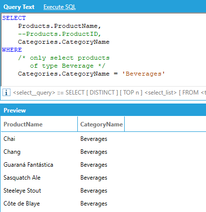
AnalytiX-BI supports comments in queries, both with the SQL single and multi-line syntax:
See Also:
AnalytiX-BI Server - Diagnostic Counters
Copyright ICONICS - version 10.97 - contact us - legal - privacy