|
|
The features on this page require a GENESIS64 Advanced license and are not available with GENESIS64 Basic SCADA . |

![]()
|
|
The features on this page require a GENESIS64 Advanced license and are not available with GENESIS64 Basic SCADA . |
![]()
The OVER clause can be used to define a window within a query result set. A window function then computes a value for each row in the window. The OVER clause can be used to easily calculate cumulative sums, moving averages and other calculations that would otherwise require complex and less efficient queries.
The syntax is:
SELECT window_function OVER (
[ PARTITION BY value_expression [ , ... n ] ]
[ ORDER BY order_by_expression [ COLLATE collation ] [ ASC | DESC ] [ , ... n ] ]
[ { ROWS| RANGE } <window frame extent> ]
) [ AS Alias] [ , ... n ]
And <window frame extent> is defined as:
<window frame extent> ::= { <window frame preceding> | <window frame between> }
<window frame between> ::= BETWEEN<window frame bound> AND<window frame bound>
<window frame bound> ::= { <window frame preceding> | <window frame following> }
<window frame preceding> ::=
{
UNBOUNDED PRECEDING
| <unsigned integer> PRECEDING
| CURRENT ROW
}
<window frame following> ::=
{
UNBOUNDED FOLLOWING
| <unsigned integer> FOLLOWING
| CURRENT ROW
}
Let’s now examine the arguments of the OVER clause more closely:
· PARTITION BY divides the query result sets into partitions. The window function is applied to each partition separately and computation restarts for each partition.
· ORDER BY defines the logical order of the rows within each partition of the result set and so determines the logical order in which the window function calculation is performed.
· ROWS / RANGE limits the rows within the partition by specifying start and end points within the partition with respect to the current row by either physical (ROWS) or logical (RANGE) association.
The window function can be either an aggregate function, a ranking function or an analytic function.
When OVER is specified with no arguments, the window function is then applied to the entire dataset. For example, the following query calculates the sum of all the units in stock for the entire Products table:
SELECT
CategoryID,
ProductName,
SUM(UnitsInStock) OVER() AS TotalUnits
FROM
Products
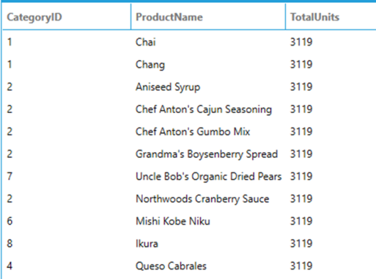
The TotalUnits value is the same for each row because the entire table is considered as a single partition, which means every row computes the same result.
Specifies the columns by which the dataset is partitioned. Expressions used in PARTITION BY can only reference columns made available by the FROM clause and cannot refer to expressions or aliases in the select list.
The following example uses PARTITION BY to split the result set in partitions before computing the window function:
SELECT
CategoryID,
ProductName,
SUM(UnitsInStock) OVER(PARTITION BY CategoryID) AS TotalUnits
FROM
Products
ORDER BY
ProductName
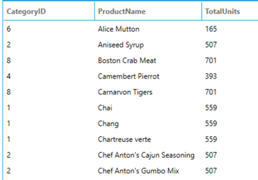
In this case since the data is partitioned by CategoryID, each row with the same CategoryID has the same result, but different partitions have different results.
Defines the logical order of the rows within each partition of the dataset. If ROWS / RANGE is not specified then the default ROWS BETWEEN UNBOUNDED PRECEDING AND CURRENT ROW is used as a default window frame by the window functions that can accept optional ROWS / RANGE specification. When a sort direction is not specified, ASC is applied.
The following example calculates the running total of Freight by CustomerID:
SELECT
CustomerID,
OrderDate,
Freight,
SUM(Freight) OVER (PARTITION BY CustomerID ORDER BY OrderDate) AS RunningTotal
FROM
Orders
WHERE
CustomerID IS NOT NULL
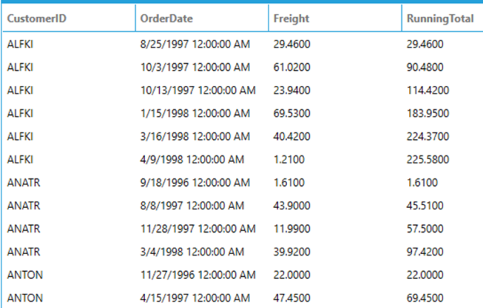
Since ROWS / RANGE is not specified, the default ROWS BETWEEN UNBOUNDED PRECEDING AND CURRENT ROW is utilized. This means that for each row, the frame that the window function uses to compute the result starts at the beginning of the partition (UNBOUNDED PRECEDING) and stops at the CURRENT ROW.
Further limits the window frame over which the window function is computed by specifying start and end points within the partition. This is accomplished by specifying a range of rows with respect to the current row either by logical (RANGE) or physical (ROWS) association.
The ROWS clause limits the rows within a partition by a fixed number of rows preceding and/or following the current row, whereas the RANGE clause logically limits the rows within a partition by specifying a range of values with respect to the value in the current row. Preceding and following rows are defined based on the ordering in the ORDER BY clause and all rows with the same values in the order by expression as the current row will be considered in the same frame (when using RANGE).
The possible values that can be used to specify a window frame are:
Specifies that the window frame starts at the first row of the partition. UNBOUNDED PRECEDING can only be used as a window starting point.
Specifies that the window frame starts at the fixed offset defined by <unsigned integer> before the current row. This specification is not allowed for RANGE.
Specifies that the window frame starts or ends at the current row, or at the current value when used with RANGE. CURRENT ROW can be used both as a starting and ending point.
Specifies that the window frame ends at the last row of the partition. UNBOUNDED FOLLOWING can only be used as a window ending point.
Specifies that the window frame ends at the fixed offset defined by <unsigned integer> after the current row. This specification is not allowed for RANGE.
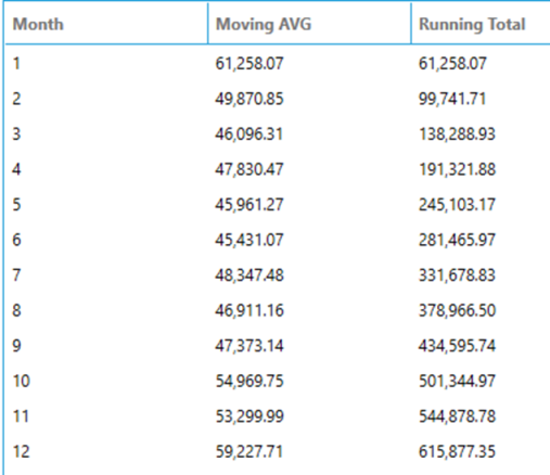
To understand the difference between ROWS and RANGE, consider the following query which sums the unit price for each product in an order:
SELECT
o.OrderDate,
o.OrderID,
SUM(UnitPrice) OVER (PARTITION BY o.OrderDate ORDER BY o.OrderID ROWS CURRENT ROW),
SUM(UnitPrice) OVER (PARTITION BY o.OrderDate ORDER BY o.OrderID RANGE CURRENT ROW)
FROM
Orders AS o
INNER JOIN
OrderDetails AS od
ON
o.OrderID = od.OrderID
WHERE
CustomerID IS NOT NULL
The window frame starts at the beginning of the partition (when omitted it defaults to UNBOUNDED PRECEDING) and, when using ROWS, the function is computed until the current physical row. For RANGE, however, all rows with the same values in the ORDER BY expression as the current row will be considered in the same frame and so computed at the same time because they are logically associated with the current physical row.
The next sections will detail which functions can be used as window functions with OVER.
Aggregates can be used to easily calculate running totals, moving averages, etc. The following query calculates the monthly order total for the year 1997 by using a subquery, and then uses window functions over this result to compute a moving average for the previous 3 months and a running total. The results are formatted with thousand separators and decimals using the toformat function.
SELECT
Month,
toformat(AVG(Total) OVER (ORDER BY [Month] ROWS BETWEEN 3 PRECEDING AND CURRENT ROW), 'n') AS [Moving AVG],
toformat(SUM(Total) OVER (ORDER BY [Month]), 'n') AS [Running Total]
FROM
(
SELECT
month(OrderDate) AS [Month],
SUM(Quantity * UnitPrice * (1 - Discount)) AS [Total]
FROM
Orders AS o INNER JOIN OrderDetails AS od ON od.OrderID = o.OrderID
INNER JOIN
Customers AS c ON c.CustomerID = o.CustomerID
WHERE
year(OrderDate) = 1997
GROUP BY
month(OrderDate)
) AS t
ORDER BY Month
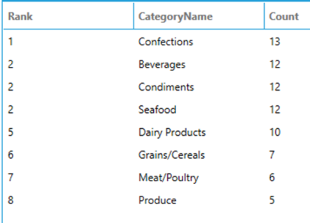
Ranking functions return a ranking value for each row in a partition. Depending on the function that is used, some rows might receive the same value as other rows. Below are the ranking functions implemented in BI SQL.
Returns the rank of each row within the partition of the dataset. The rank of a row is one plus the number of ranks that come before the row in question. If two or more rows tie for a rank (i.e.: they have the same value of the ORDER BY expression), each tied row receives the same rank. The next row that is not tied will receive the previous rank plus the number in the previous rank as its own rank.
The following query ranks categories based on the number of products that belong to them. Notice that categories with the same number of products have the same rank.
SELECT
RANK() OVER (ORDER BY [Count] DESC) AS [Rank],
CategoryName,
[Count]
FROM
(
SELECT
COUNT(*) AS [Count],
CategoryName
FROM
Products AS p INNER JOIN Categories AS c ON p.CategoryID = c.CategoryID
GROUP BY
CategoryName
) AS t
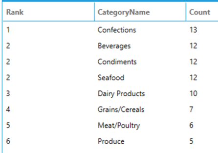
This function returns the rank of each row within a partition with no gaps in the ranking values. The rank of a specific row is one plus the number of distinct rank values that come before that specific row. If two or more rows tie for a rank (i.e.: they have the same value of the ORDER BY expression), each tied row receives the same rank. The next row that is not tied will receive the number of distinct rows that come before the row in question plus one as its own rank.
The following query dense ranks categories based on the number of products that belong to them.
SELECT
DENSE_RANK() OVER (ORDER BY [Count] DESC) AS [Rank],
CategoryName,
[Count]
FROM
(
SELECT
COUNT(*) AS [Count],
CategoryName
FROM
Products AS p INNER JOIN Categories AS c ON p.CategoryID = c.CategoryID
GROUP BY
CategoryName
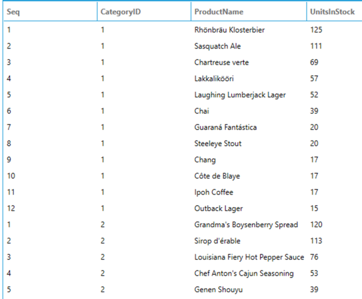
Numbers the output of a result set by returning the sequential number of a row within a partition of a dataset, starting at 1 for the first row in each partition.
Note: there is no guarantee that the rows returned by a query using ROW_NUMBER will be ordered exactly the same within each execution unless the following conditions are true:
1. Values of the partitioned column are unique
2. Values of the ORDER BY columns are unique
3. Combinations of values of the partition column and ORDER BY columns are unique
The following query assigns a sequence number to products partitioned by CategoryID and ordered by UnitsInStock:
SELECT
ROW_NUMBER() OVER (PARTITION BY CategoryID ORDER BY UnitsInStock DESC) AS [Seq],
CategoryID,
ProductName,
UnitsInStock
FROM
Products
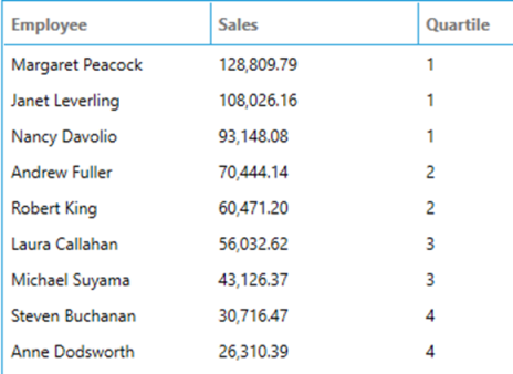
Distributes rows in a partition into the specified number of groups, numbered starting at one. For each row, NTILE returns the number of the group to which the row belongs. If the number of rows in the dataset is not divisible by the number of desired groups, it will cause groups of two sizes that differ by one member. Larger groups come before smaller groups in the order specified by the OVER clause. For example, if the dataset number of rows is 13 and the number of groups is 3, the first group will have 5 rows and the remaining two groups will have 4 rows.
The following query divides employees into four groups based on sales for the year 1997.
SELECT
Employee,
toformat(Sales, 'n') AS Sales,
NTILE(4) OVER (ORDER BY Sales DESC) AS Quartile
FROM
(
SELECT
SUM(Quantity * UnitPrice * (1 - Discount)) AS Sales,
FirstName + ' ' + LastName AS Employee
FROM
Orders AS o INNER JOIN OrderDetails AS od ON o.OrderID = od.OrderID
INNER JOIN
Employees AS e ON e.EmployeeID = o.EmployeeID
WHERE
year(OrderDate) = 1997
) AS t
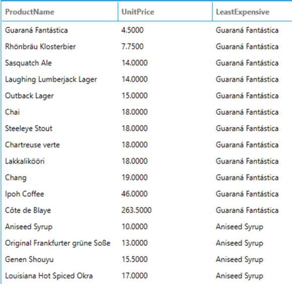
These functions can return values at specific places in a window frame.
Returns the first value in the current window frame. The following query returns the list of products, their unit price and the least expensive product in the same category. Note that the least expensive product is fixed for each partition because the frame always starts at the first row (when omitted, it defaults to UNBOUNDED PRECEDING).
SELECT
ProductName,
UnitPrice,
FIRST_VALUE(ProductName) OVER (PARTITION BY CategoryID ORDER BY UnitPrice) AS LeastExpensive
FROM
Products
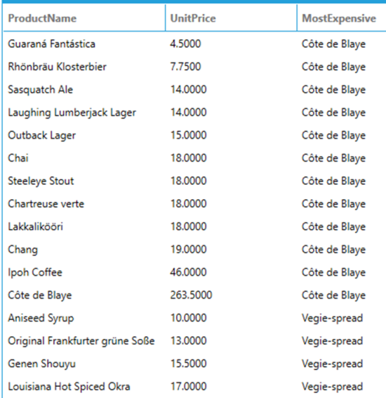
Returns the last value in the current window frame. The following query returns the list of products, their unit price and the most expensive product in the same category. Note that the most expensive product is fixed for each partition because the frame ends at UNBOUNDED FOLLOWING.
SELECT
ProductName,
UnitPrice,
LAST_VALUE(ProductName) OVER (PARTITION BY CategoryID ORDER BY UnitPrice ROWS BETWEEN CURRENT ROW AND UNBOUNDED FOLLOWING) AS MostExpensive
FROM
Products
ORDER BY
CategoryID, UnitPrice
Returns the value from a previous row in the same dataset, which allows to compare the current row with a previous row. By default, LAG returns the value of the row immediately preceding the current row, however a custom offset can be specified as the second, optional, parameter of the function. A third optional parameter can be used to specify a default value to return when the value being retrieved by LAG falls outside of the window frame: if this parameter is not specified then NULL is used as a default value. Both offset and default value can be a constant, a column reference or an expression.
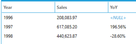
The following query calculates yearly sales using a subquery and then uses LAG on the result in order to compute the year over year change.
SELECT
[Year],
toformat(Sales, 'n') AS Sales,
toformat((Sales / (LAG(Sales) OVER (ORDER BY [Year] ASC)) - 1) * 100, 'n') + '%' AS YoY
FROM
(
SELECT
year(OrderDate) AS [Year],
SUM(Quantity * UnitPrice * (1 - Discount)) AS [Sales]
FROM
Orders AS o INNER JOIN OrderDetails AS od ON od.OrderID = o.OrderID
GROUP BY
year(OrderDate)
) AS t
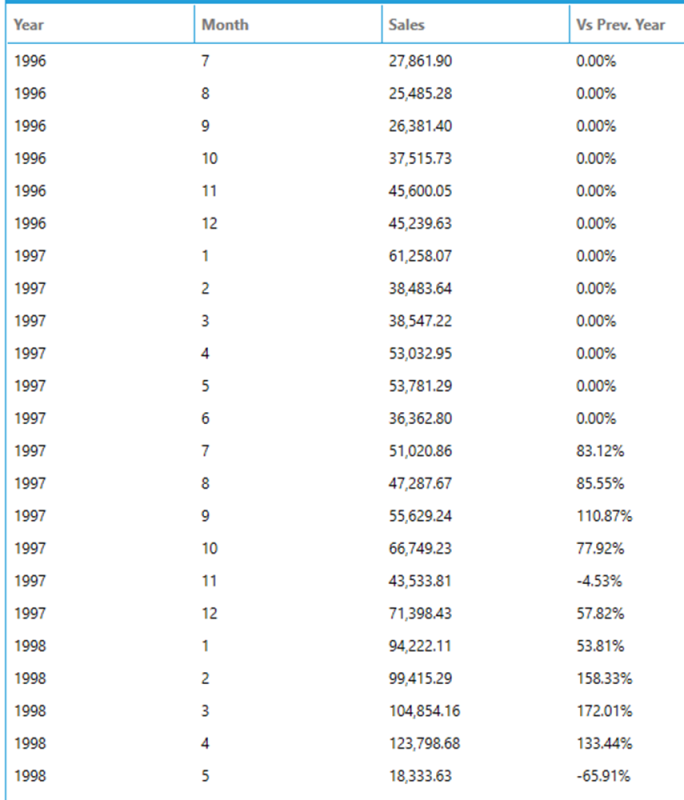
The following query calculates monthly sales using a subquery and then uses LAG on the result in order to compute a month over the same month of the previous year change using 12 as an offset for the LAG function. The example also uses the value of Sales as the default value so that the change results in 0 when a month to calculate the comparison does not exist.
SELECT
[Year],
[Month],
toformat(Sales, 'n') AS Sales,
toformat((Sales / (LAG(Sales, 12, Sales) OVER (ORDER BY [Year] ASC)) - 1) * 100, 'n') + '%' AS [Vs Prev. Year]
FROM
(
SELECT
year(OrderDate) AS [Year],
month(OrderDate) AS [Month],
SUM(Quantity * UnitPrice * (1 - Discount)) AS [Sales]
FROM
Orders AS o INNER JOIN OrderDetails AS od ON od.OrderID = o.OrderID
GROUP BY
year(OrderDate),
month(OrderDate)
) AS t
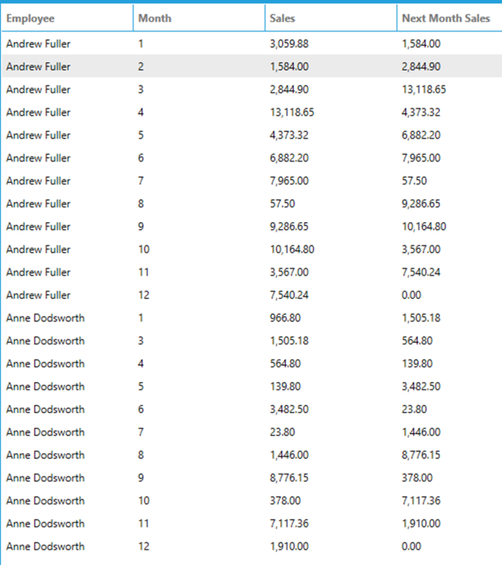
Returns the value from a following row in the same dataset. By default, LEAD returns the value of the row immediately following the current row, however a custom offset can be specified as the second, optional, parameter of the function. A third optional parameter can be used to specify a default value to return when the value being retrieved by LEAD falls outside of the window frame: if this parameter is not specified then NULL is used as a default value. Both offset and default value can be a constant, a column reference or an expression.
The following query calculates monthly sales by employee for the year 1997 and then uses the LEAD function partitioned by Employee and sorted by month to show the next month sales per employee.
SELECT
[Employee],
[Month],
toformat(Sales, 'n') AS Sales,
toformat(LEAD(Sales, 1, 0) OVER (PARTITION BY Employee ORDER BY [Month] ASC), 'n') AS [Next Month Sales]
FROM
(
SELECT
e.FirstName + ' ' + e.LastName AS Employee,
month(OrderDate) AS [Month],
SUM(Quantity * od.UnitPrice * (1 - Discount)) AS [Sales]
FROM
Orders AS o INNER JOIN OrderDetails AS od ON od.OrderID = o.OrderID
INNER JOIN
Employees AS e ON e.EmployeeID = o.EmployeeID
WHERE
year(OrderDate) = 1997
GROUP BY
e.FirstName + ' ' + e.LastName,
month(OrderDate)
) AS t